A function is a predefined formula that performs calculations using specific values in a particular order. Excel includes many common functions that can be used to quickly find the sum, average, count, maximum value, and minimum value for a range of cells. In order to use functions correctly, you'll need to understand the different parts of a function and how to create arguments to calculate values and cell references.
Watch the video below to learn more about working with functions.
The parts of a function
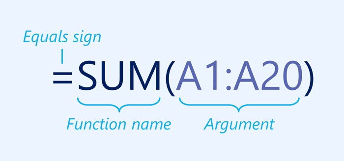
In order to work correctly, a function must be written a specific way, which is called the syntax. The basic syntax for a function is the equals sign (=), the function name (SUM, for example), and one or more arguments. Arguments contain the information you want to calculate. The function in the example below would add the values of the cell range A1:A20.
Working with arguments
Arguments can refer to both individual cells and cell ranges and must be enclosed within parentheses. You can include one argument or multiple arguments, depending on the syntax required for the function.
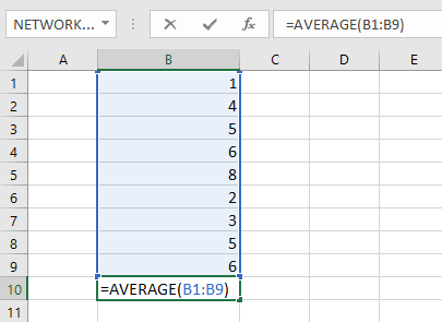
For example, the function =AVERAGE(B1:B9) would calculate the average of the values in the cell range B1:B9. This function contains only one argument.
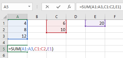
Multiple arguments must be separated by a comma. For example, the function =SUM(A1:A3, C1:C2, E1) will add the values of all of the cells in the three arguments.
Creating a function
There are a variety of functions available in Excel. Here are some of the most common functions you'll use:
SUM: This function adds all of the values of the cells in the argument.
AVERAGE: This function determines the average of the values included in the argument. It calculates the sum of the cells and then divides that value by the number of cells in the argument.
COUNT: This function counts the number of cells with numerical data in the argument. This function is useful for quickly counting items in a cell range.
MAX: This function determines the highestcell value included in the argument.
MIN: This function determines the lowest cell value included in the argument.
To create a function using the AutoSum command:
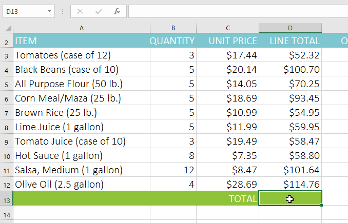
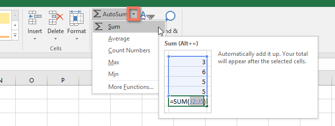
The AutoSum command allows you to automatically insert the most common functions into your formula, including SUM, AVERAGE, COUNT, MAX, and MIN. In the example below, we'll use the SUM function to calculate the total cost for a list of recently ordered items.
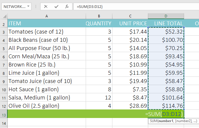
Select the cell that will contain the function. In our example, we'll select cell D13.
In the Editing group on the Home tab, click the arrow next to the AutoSum command. Next, choose the desired function from the drop-down menu. In our example, we'll select Sum.
Excel will place the function in the cell and automatically select a cell range for the argument. In our example, cells D3:D12 were selected automatically; their values will be added to calculate the total cost. If Excel selects the wrong cell range, you can manually enter the desired cells into the argument.
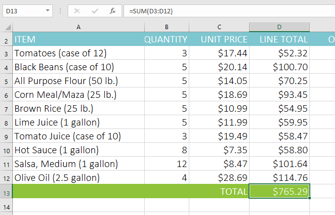
Press Enter on your keyboard. The function will be calculated, and the result will appear in the cell. In our example, the sum of D3:D12 is $765.29.
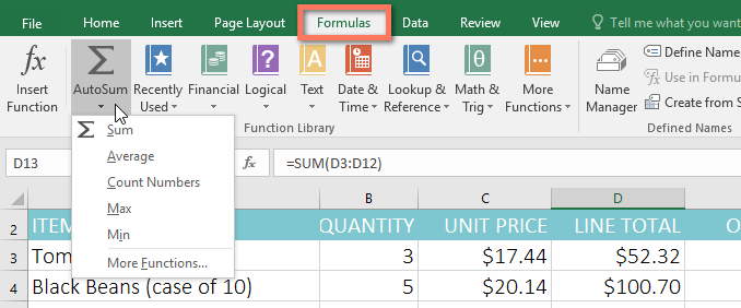
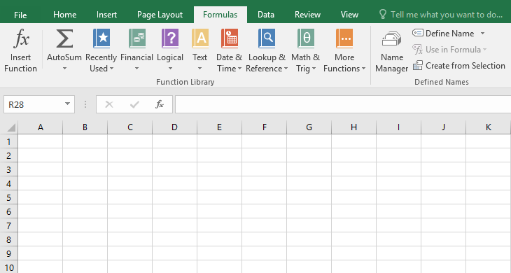
The AutoSum command can also be accessed from the Formulas tab on the Ribbon.
You can also use the Alt+= keyboard shortcut instead of the AutoSum command. To use this shortcut, hold down the Alt key and then press the equals sign.
Watch the video below to see this shortcut in action.
To enter a function manually:
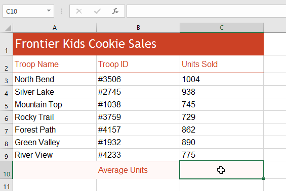
If you already know the function name, you can easily type it yourself. In the example below (a tally of cookie sales), we'll use the AVERAGE function to calculate the average number of units sold by each troop.
Select the cell that will contain the function. In our example, we'll select cell C10.
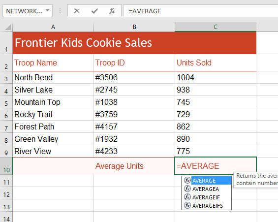
Type the equals sign (=), then enter the desired function name. You can also select the desired function from the list of suggestedfunctions that appears below the cell as you type. In our example, we'll type =AVERAGE.
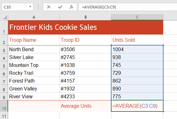
Enter the cell range for the argumentinside parentheses. In our example, we'll type (C3:C9). This formula will add the values of cells C3:C9, then divide that value by the total number of values in the range.
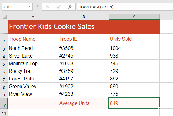
Press Enter on your keyboard. The function will be calculated, and the result will appear in the cell. In our example, the average number of units sold by each troop is 849.
Excel will not always tell you if your formula contains an error, so it's up to you to check all of your formulas. To learn how to do this, read the Double-Check Your Formulas lesson from our Excel Formulas tutorial.
The Function Library
While there are hundreds of functions in Excel, the ones you'll use the most will depend on the type of data your workbooks contain. There's no need to learn every single function, but exploring some of the different types of functions will help as you create new projects. You can even use the Function Library on the Formulas tab to browse functions by category, including Financial, Logical, Text, and Date & Time.
To access the Function Library, select the Formulas tab on the Ribbon. Look for the Function Library group.
Click the buttons in the interactive below to learn more about the different types of functions in Excel.
edit hotspots
AutoSum Command
The AutoSum command allows you to automatically return results for common functions like SUM, AVERAGE, and COUNT.
Recently Used
The Recently Used command gives you access to functions you've recently worked with.
Financial
The Financial category contains functions for financial calculations like determining a payment (PMT) or interest rate for a loan (RATE).
Logical
Functions in the Logical category check arguments for a value or condition. For example, if an order is more than $50, add $4.99 for shipping; if it is more than $100, do not charge for shipping (IF).
Text
The Text category contains functions that work with the text in arguments to perform tasks, such as converting text to lowercase (LOWER) or replacing text (REPLACE).
Date & Time
The Date & Time category contains functions for working with dates and time and will return results like the current date and time (NOW) or the seconds (SECOND).
Lookup & Reference
The Lookup & Reference category contains functions that will return results for finding and referencing information. For example, you can add a hyperlink to a cell (HYPERLINK) or return the value of a particular row and column intersection (INDEX).
Math & Trig
The Math & Trig category includes functions for numerical arguments. For example, you can round values (ROUND), find the value of Pi (PI), multiply (PRODUCT), and subtotal (SUBTOTAL).
More Functions
More Functions contains additional functions under categories for Statistical, Engineering, Cube, Information, and Compatibility.
Insert Function
If you're having trouble finding the right function, the Insert Function command allows you to search for functions using keywords.
To insert a function from the Function Library:
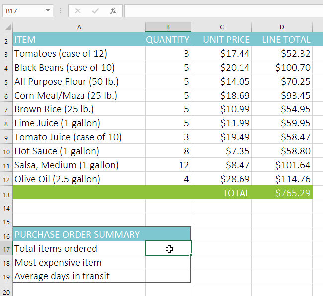
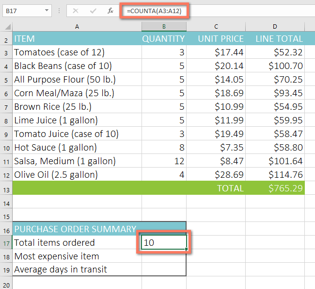
In the example below, we'll use the COUNTA function to count the total number of items in the Items column. Unlike COUNT, COUNTA can be used to tally cells that contain data of any kind, not just numerical data.
Select the cell that will contain the function. In our example, we'll select cell B17.
Click the Formulas tab on the Ribbon to access the Function Library.
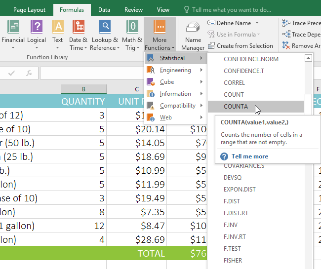
From the Function Library group, select the desired function category. In our example, we'll choose More Functions, then hover the mouse over Statistical.
Select the desired function from the drop-down menu. In our example, we'll select the COUNTA function, which will count the number of cells in the Items column that are not empty.
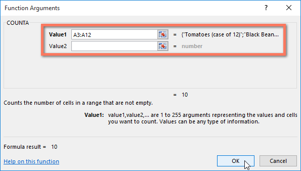
The Function Arguments dialog box will appear. Select the Value1 field, then enter or select the desired cells. In our example, we'll enter the cell range A3:A12. You can continue to add arguments in the Value2 field, but in this case we only want to count the number of cells in the cell range A3:A12.
When you're satisfied, click OK.
The function will be calculated, and the result will appear in the cell. In our example, the result shows that 10 items were ordered.
The Insert Function command
While the Function Library is a great place to browse for functions, sometimes you may prefer to search for one instead. You can do so using the Insert Function command. It may take some trial and error depending on the type of function you're looking for, but with practice the Insert Function command can be a powerful way to find a function quickly.
To use the Insert Function command:
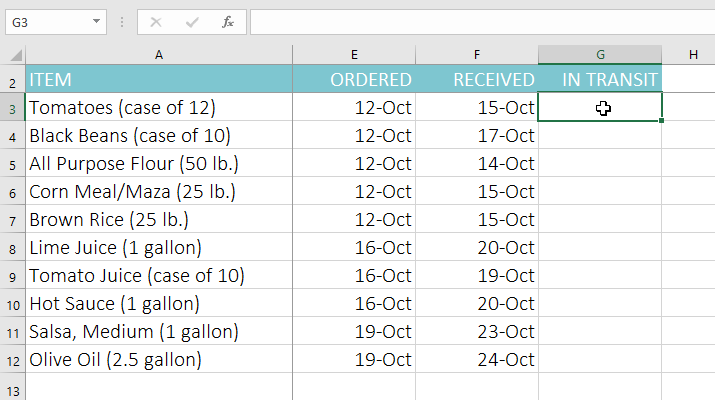
In the example below, we want to find a function that will calculate the number of business days it took to receive items after they were ordered. We'll use the dates in columns E and F to calculate the delivery time in column G.
Select the cell that will contain the function. In our example, we'll select cell G3.
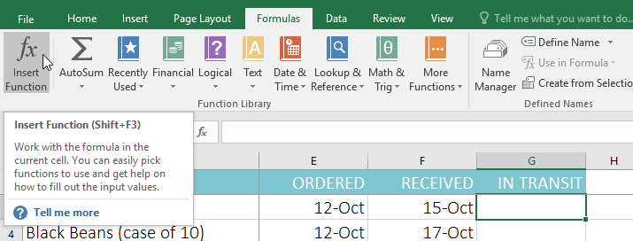
Click the Formulas tab on the Ribbon, then click the Insert Function command.
The Insert Function dialog box will appear.
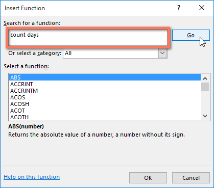
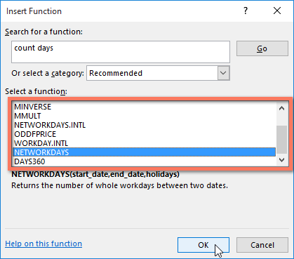
Type a few keywords describing the calculation you want the function to perform, then click Go. In our example, we'll type count days, but you can also search by selecting a category from the drop-down list.
Review the results to find the desired function, then click OK. In our example, we'll choose NETWORKDAYS, which will count the number of business days between the ordered date and received date.
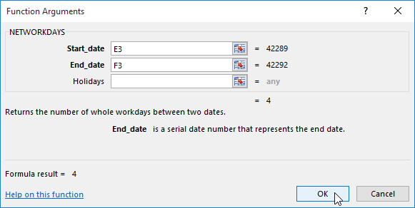
The Function Arguments dialog box will appear. From here, you'll be able to enter or select the cells that will make up the arguments in the function. In our example, we'll enter E3 in the Start_date field and F3 in the End_date field.
When you're satisfied, click OK.
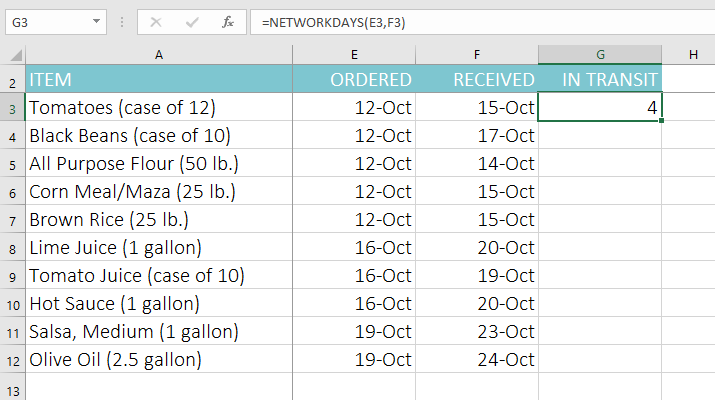
The function will be calculated, and the result will appear in the cell. In our example, the result shows that it took four business days to receive the order.
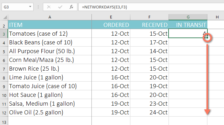
Like formulas, functions can be copied to adjacent cells. Simply select the cell that contains the function, then click and drag the fill handle over the cells you want to fill. The function will be copied, and values for those cells will be calculated relative to their rows or columns.
To learn more:
If you're comfortable with basic functions, you may want to try a more advanced one like VLOOKUP. Review our lesson on How to Use Excel's VLOOKUP Function for more information.
To learn even more about working with functions, visit our Excel Formulas tutorial.
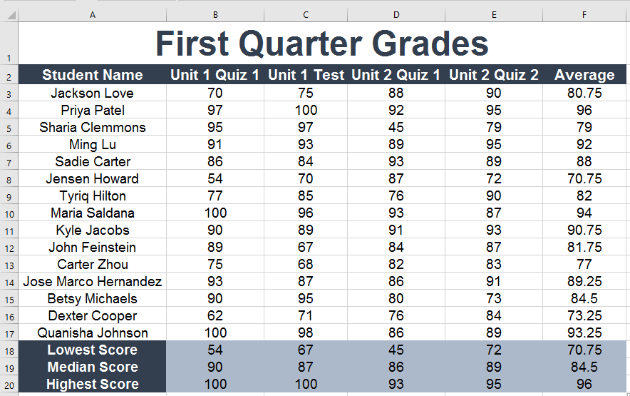
Click the Challenge tab in the bottom-left of the workbook.
In cell F3, insert a function to calculate the average of the four scores in cells B3:E3.
Use the fill handle to copy your function in cell F3 to cells F4:F17.
In cell B18, use the AutoSum command to insert a function that calculates the lowest score in cells B3:B17.
In cell B19, use the Function Library to insert a function that calculates the median of the scores in cells B3:B17. Hint: You can find the median function by going to More Functions > Statistical.
In cell B20, create a function to calculate the highest score in cells B3:B17.
Select cells B18:B20, then use the fill handle to copy all three functions you just created to cells C18:F20.
When you're finished, your workbook should look like this: