Introduction

By the end of this lesson, you should be able to:

• Apply fonts
• Apply a font color
• Apply borders

Changing font type, size, and color

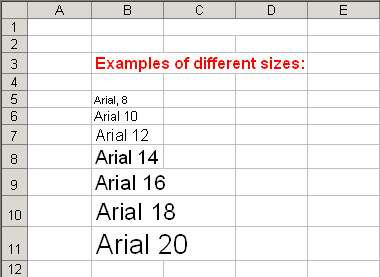
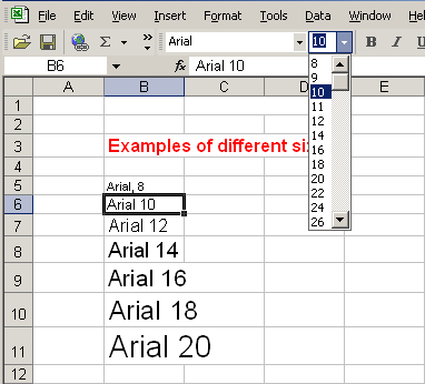
In Excel XP, a font consists of three elements: typeface, or the style of the letter; size of the letter; and color of the letter. The default font in a spreadsheet is Arial 10 points, but the typeface and size can be changed easily.

Selecting a font typeface

The amount of typefaces available for use varies depending on the software installed on your computer.

To apply a typeface to information in a cell:

• Select a cell or range of cells.
• Click the down arrow to the right of the Font Name list box on the Formatting toolbar.
  
  
• A drop-down list of available fonts appears.
  
  
• Click the typeface of your choice.
• The selection list closes, and the new font is applied to the selected cells.

Changing font type, size, and color

To apply a font size to information in a cell:

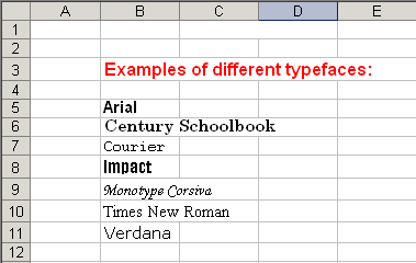
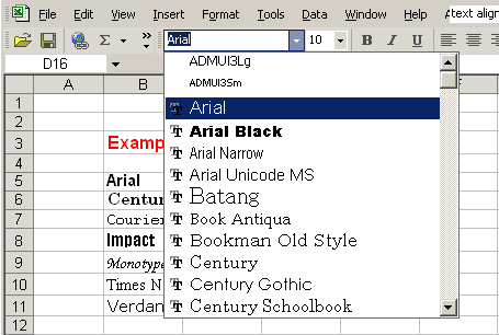
The font size list varies from typeface to typeface. The Arial font sizes, for example, are 8, 9, 10, 11, 12, 14, 16, 18, 20, 22, 24, 26, 28, 36, 48, and 72.

• Select a cell or range of cells.
• Click the down arrow to the right of the font size list box on the Formatting toolbar.
  
  
• A drop-down list of available font sizes appears.
  
  
• Click the font size of your choice.
• The selection list closes, and the new font size is applied to the selected cells.

Changing font type, size, and color

To apply color to information in cells:

• Select a cell or range of cells.
• Click the down arrow to the right of the font color list box.
  
  
• A drop-down list of available colors appears.
  
  
• Click the color of your choice.
• The selection list closes, and the new font color is applied to the selected cells.

Using underline, italics, and bold

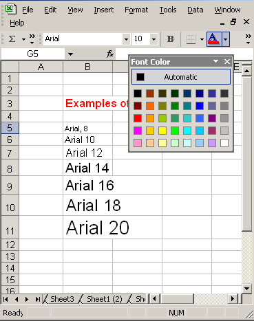
In addition to the typeface, size and color, you can apply bold, italics, and/or underline font style attributes to any text or numbers in cells.

To select a font style:

• Select a cell or range of cells.
• Click any of the following options on the Formatting toolbar:
  
  
• Bold (Ctrl+B)
• Italics (Ctrl+I)
• Underline (Ctrl+U)
• The attribute(s) selected are applied to the font.

The bold, italics, and underline buttons on the Formatting toolbar are like toggle switches: Click once to turn one on, and click again to turn it off.

Designing and applying styles

Styles can save a lot of time when formatting a spreadsheet. A style is a unique collection of font attributes that include number, alignment, font, border, patterns, and protection. Many different styles can be created in a spreadsheet, each with different attributes and names. When applied to a cell, information in it resembles the attributes defined for that style.

To apply a style:

• Select the cell or range of cells.
• Choose FormatStyle from the menu bar.
  
  
• Select a style from the Style name drop-down list.
  
  

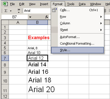
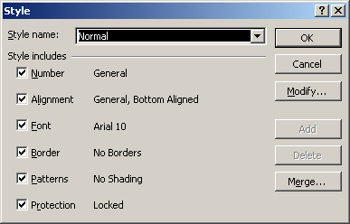
You can change the style attributes for any style name.

You can create new styles by clicking the Add button in the Style dialog box.

Adding a border to cells

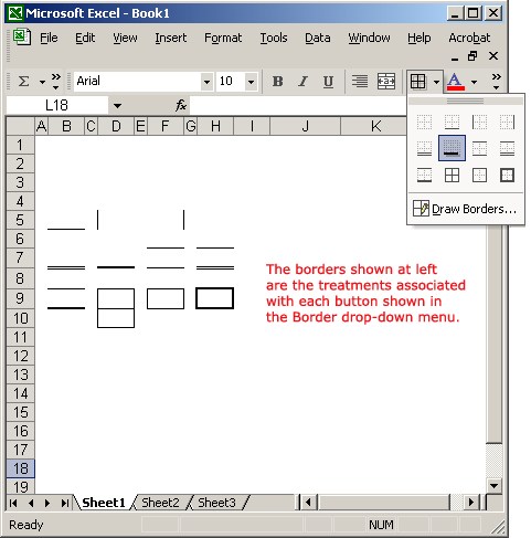
Borders can be applied to cells in your worksheet to emphasize important data or assign names to columns or rows.

To add a border to a cell or cell range:

• Select a cell or range of cells.
• Click the down arrow next to the Borders button.
• The Border drop-down menu appears.
  
  
• Choose a border line style from the Border drop-down menu.
  
  
• The selected cells display the chosen border.

Adding color to cells

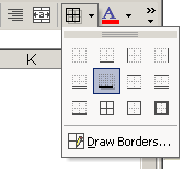
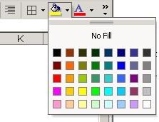
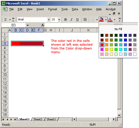
Colors can be applied to cells in your worksheet to emphasize important data or assign names to columns or rows.

To add color to a cell:

• Select a cell or range of cells.
• Click the down arrow next to the font color button. A font color drop-down menu displays.
  
  
• Choose a color from the font color drop-down menu.
  
  
• The selected cells display the color.

Challenge!

• Type the label Learning about fonts in Excel in cell B2.
• Change the font in cell B2 to have a typeface of Times New Roman, a size of 16, and a color of red.
• Type the word Underline in cell B3 and apply an underline treatment to it.
• Type the word Italics in cell B4 and apply an italics treatment to it.
• Type the word Bold in cell B3 and apply a bold treatment to it.
• Select a cell range that includes cells B2, B3, B4, and B5.
• Add a border around the cell range.
• Define a color of yellow around the cell range.